
Introduction to Darfix (6.x)#
darfix is a Python library for the analysis of dark-field microscopy data. darfix is to be used as a workflow, together with a graphical user interface based on Orange3.
The aim of this tutorial is to guide you into correctly executing darfix into a correct analysis of your images.
This tutorial will show how to use the 3 main darfix parts:
Load the data and select the different motors (dimensions). Select a transformation technique (RSM, magnification), if needed.
Pre-analysis of the images by applying several operations like region of interest, noise removal and shift correction.
- Apply DFXM analysis to the images. The DFXM techniques currently in darfix are
Rocking curve imaging: Fits the data along the z-dimension (pixel by pixel) according to a Gaussian distribution. After computation, the maps of the fit parameters will be shown. The fitted data is saved on disk in HDF5 format.
Grain plot: Several maps are plotted which can be exported into a single file: COM, FWHM, skewness, kurtosis (for every dimension). There is also mosaicity and orientation distribution maps in case of 2D datasets.
Blind source separation: An experimental technique that uses different blind source separation techniques to find grains along the dataset, tests with different datasets have shown good results with techniques like NMF, NNICA, and NMF+NNICA.
Pre-requisites#
The data format should either HDF5 or EDF.
Warning
EDF is a legacy format and will no longer be supported natively starting from Darfix 4.0.
However, it is possible to convert EDF to HDF5 to load the data in Darfix.
- Motor information should be contained in metadata.
For HDF5: a group should contain all positioners datasets.
for EDF: headers should contain motors_mne information.
The data should be a stack of images (dimensions: N_frames x W x H).
Installing darfix#
At ESRF#
darfix is already installed on the SLURM cluster. To run it, follow these steps:
Connect to the cluster
ssh -X cluster-access
Request an interactive job on a node with appropriate resources
salloc -p interactive –x11 srun –pty bash
Load the darfix module
module load darfix
Launch darfix
darfix
The following window should then appear:
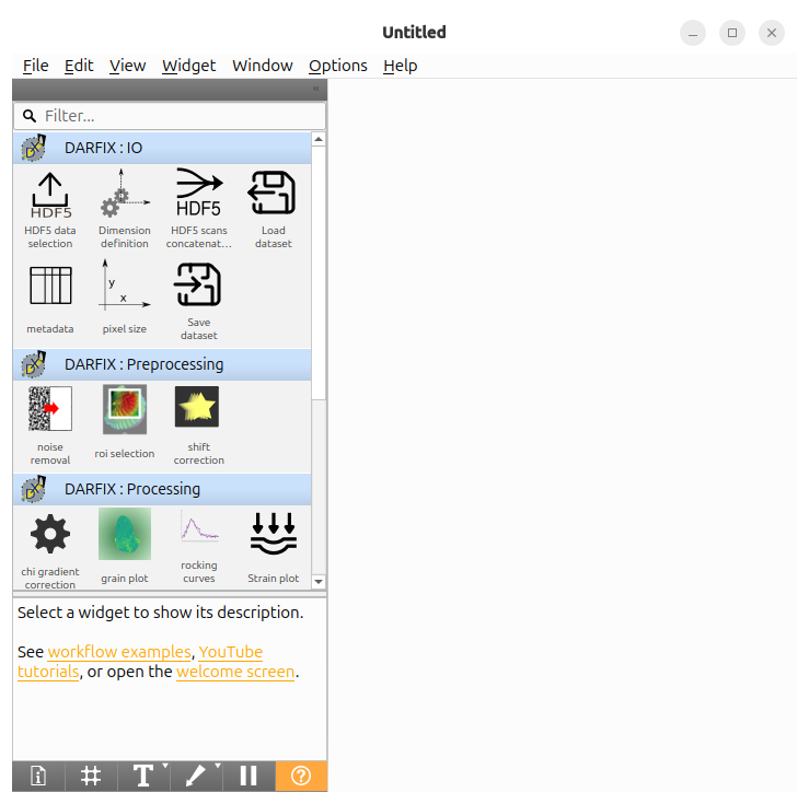
Outside ESRF#
Install darfix according to the instructions in Installation
Then, you can launch darfix by running
darfix
and get the same window as above.
Workflow creation#
To get a workflow quickly, you can start from one of the workflow examples.
Help > Example Workflows
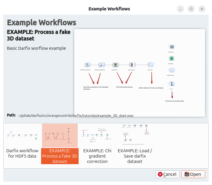
Three example workflows are available.
For quick start, have a look at EXAMPLE: Process a fake 3D dataset.
The preprocessing chain is already wired up and the inputs are pre-filled.
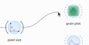
You only need to connect the last widget to the analysis widget you want to try (grain plot, rocking curves, z-sum or strain plot).
Draw a link by clicking on the output port of the last connected widget and dragging it to the target widget:
Tip
To navigate through a workflow:
After configuring a widget, click OK to validate and pass data to the next widget.
For preprocessing widgets (ROI Selection, Noise Removal), click Apply first to preview the result, then OK to confirm.